The Explosion of CRISPR-Cas9
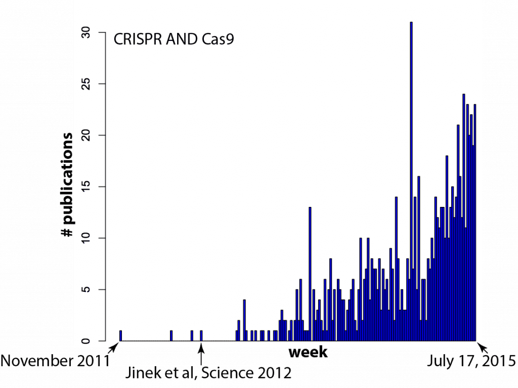
It seems like every time you turn around, there’s another paper that mentions CRISPR-Cas9. Just how fast has the field exploded? There’s nothing like data to find out! In the histogram below, each bar on the X-axis is a week (arbitrarily starting in late 2011) and the Y-axis is the number of papers in a Pubmed search for “CRISPR AND Cas9” (side note: one needs to include CRISPR in the search because “Cas9” spuriously includes results from a few labs that like to call caspases “Cas”, e.g. caspase 9 = Cas9, caspase 3 = Cas3).
Your hunch was correct — there IS a new paper mentioning CRISPR/Cas9 every time you turn around: several per day, in fact.
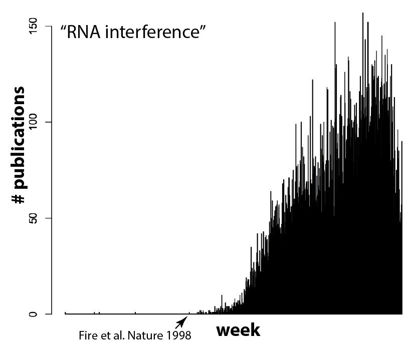
And I think (hope) that means we’re reaching a tipping point. It’s currently in vogue to sprinkle “Cas9” throughout a paper, even if the system is used as tool for biology and not itself the focus of the work, because it gets the attention of editors. But as more and more groups use Cas9, gene editing will become commonplace. Routine, even. And that’s exactly what should happen! Can you imagine a paper these days that crows about how they used gel electrophoresis to separate proteins, or PCR and restriction enzymes to clone a gene? It’s the natural course of things for disruptive technologies to quickly become just another part of the toolbox. RNAi for example, which completely upended biology not too long ago and is now used routinely and without fuss by most cell biology labs. Compare the plot above with the equivalent for RNAi (the search here was for “RNA interference” due to complications in searching “RNAi”, since that also finds other hits on a viral RNA called “RNA-one”. Also note that there are some false positives before Andy Fire’s 1998 Nature paper).
I’m looking forward to the day that CRISPR-Cas9 becomes as common-place as RNAi, since it will mean we’ve arrived at a new another era of biology. Want to know what that conserved genetic element does? Just remove it. Want to find out what that conserved residue does in your favorite protein? Mutate it in your organism of interest. No big deal!
That’s going to be an incredible time. I’m in this for the destination, not the vehicle.
For those interested, here’s how to generate the histogram
(download medline format records for a pubmed search)
# medlinedates.py
#!/usr/bin/env python
from Bio import Medline # requires Biopython
import datetime
import sys
fin = sys.argv[1]
with open(fin) as p:
records = Medline.parse(p)
for record in records:
d = record['DA']
d = datetime.date(int(d[:4]), int(d[4:6]), int(d[6:8]))
print d.toordinal()
—-
(on the command line)
$ medlinedates.py [medline format file you downloaded] > dates.txt
—-
(in R)
# plotdates.R
d<-read.table("dates.txt", header=F)
ranges<-append(c(seq(min(d$V1), max(d$V1), by = 7)), max(d$V1))
hist(d$V1, breaks=ranges, freq=TRUE, col="blue")
You may also be interested in
Protected: Announcing the Rising Stars Program: A New Collaboration Between the IGI and Historically Black Colleges and Universities
Breakthrough Method Enables Rapid Discovery of New Useful Proteins

From California to Kenya: The 2025 Cohort of the CRISPR Course for African Plant Scientists

 By
Jacob Corn